Moore-Penrose Pseudoinverse

Generalization of the inverse of a matrix.

I believe, we pay too much attention to implementation, and too less
attention in the study of the concept that is implemented. I have been
on then teams of many Data Science and Machine Learning projects, and
I would always reiterate on one simple idea; that is, “If you do not
know the math, you don’t know it at all.”

This is a piece of philosophy I deeply believe in. With the advent of packages like numpy, matplotlib, scikit-learn etc., implementing a machine learning model with a moderately difficult data set and problem is fairly simple.
The magic then stays in being able to tweak the algorithm and getting something new (or weird) out of the model. And, for you to be capable of doing so, you will have to know the mechanism behind it.
The Moore-Penrose pseudoinverse in the soul of PCA (Principal Component Analysis), one of the most popularly used Dimensionality reduction techniques.

---

How do we define the inverse of a matrix?
Provided that the matrix is a square matrix and non-singular, we simple divide the adjoint of the matrix with its determinant.
Mathematically, for $A_{m \times m}$ and $|A| \neq 0$, the inverse of $A$ is defined as,
$$A^{-1} = \frac{ \text{adj.} A}{|A|} \tag*{(1)}$$

---

Of course, the above method is computationally very expensive. Hence, we can get the inverse of the matrix recursively using the Fadeev-LeVerrier equation ( Read about that in this blog of mine).

---

Now, how do we deal with matrices that are non-square? How do you find the inverse of a matrix that looks like this,
$$B = \begin{bmatrix} x_{11} & x_{13} \\ x_{21} & x_{23}\\ x_{d1} & x_{d3} \end{bmatrix}_{3\times 2}$$
This is where the Generalization of inverse of a matrix happens, named the Moore-Penrose Pseudoinverse.

---

For every $A_{m \times n}$, there exists a pseudoinverse $A^{\dagger}_{n \times m}$. ( $A^\dagger$ is read as “A dagger”).
$A^{\dagger}$ is mathematically defined as,
$$A^{\dagger}=(A^{T}A)^{-1}A^{T} \tag*{(2)}$$
This is dimensionally consistent. Please check and verify.

---

Now, say we have,
$$Q = \begin{bmatrix} 1 \\ 2 \end{bmatrix}$$
It is impossible to find $Q^{-1}$ by the conventional method $(1)$. So, we use the Generalized Inverse at $(2)$.
So,
$$Q^{T} = \begin{bmatrix} 1 && 2 \end{bmatrix}$$
So, $Q^{T}Q$ comes out to be $[5]_{1 \times 1}$. So, $(Q^{T}Q)^{-1}$ comes out to be $\frac{1}{5}$.
Hence,
$$Q^{\dagger}=(Q^{T}Q)^{-1}Q^{T} =\frac{1}{5} \begin{bmatrix} 1 && 2 \end{bmatrix} = \begin{bmatrix} \frac{1}{5} && \frac{2}{5} \end{bmatrix}$$ which is the pseudoinverse or the generalized inverse.

---

For a square matrix (i.e., $m \times m$),
$$A^{\dagger}=A^{-1}$$
In detail,
$$(A^{T}A)^{-1}A^{T}=\frac{\text{adj. A}}{|A|}$$

---

Some properties of the generalized inverse are,
1. $AA^{\dagger}A=A$
2. $A^{\dagger}AA^{\dagger}=A^{\dagger}$
3. $(AA^{\dagger})=AA^{\dagger}$
One important point to remember is, $A^{\dagger}$ always exists and is unique.

---

Cheers!

The Linear Quadratic Regulator

Optimal Control and Linear-Quadratic-Regulator (LQR)

Today, I will not write an introductory passage to write off my blog. Because, writing an introduction to Optimal Control in itself will required a blog. However, I will add in small tidbits as and when needed.
To understand the topic, we need some basic definitions with us.

---

1.
A control system can be represented in terms of State Space, as follows,
$$\boxed{\dot{x}(t) = A(t)x(t)+B(t)u(t) \\ y(t)=C(t)x(t)+D(t)u(t)}$$
In the above formulation,
$x(.)$ is the state vector; $x(t) \in \mathcal{R}^{n}$.
$y(.)$ is the output vector; $y(t) \in \mathcal{R}^{q}$.
$u(.)$ is the input vector; $u(t) \in \mathcal{R}^{p}$.
$A(.)$ is the System Matrix; $\mathrm{dim}[A(.)]=n\times n$.
$B(.)$ is the Input Matrix; $\mathrm{dim}[B(.)]=n\times p$.
$C(.)$ is the Output Matrix; $\mathrm{dim}[C(.)]=q\times n$.
$A(.)$ is the Feed-forward Matrix; $\mathrm{dim}[D(.)]=q\times p$.
Now, for a system to be controllable, we first define a matrix $\mathcal{Q_c}$, called the controllability matrix, such that,
$$\boxed{\mathcal{Q}_c=\begin{bmatrix} B & AB & A^{2}B & \ldots & A^{n-1}B \\ \end{bmatrix}}$$
The system is controllable if $\mathcal{Q}_c$ has full row rank (i.e. rank($\mathcal{Q}_c$) $=n$).

---

We will assume that we deal with Controllable systems only.

---

Usually, a single input system’s state feedback controller is designed using the Eigen-value method, or Pole Placement method.

---

2.
Pole placement method is the methodology of finding the control vector $\mathcal{U}$ in the form $-\mathcal{k}x$
So, the state space representation changes as,
$$\dot{x}=(A-Bk)x$$
$k$ is found as,
$$|sI-(A-Bk)|=(s-\mu_1)(s-\mu_2)...(s-\mu_n)$$
Here, $\mu$ are the desired pole locations. Note that $k$ is defined as $k=\begin{bmatrix} k_1 & k_2 & k_3 & \ldots & k_n\ \end{bmatrix}$

---

However, for a multi-input system the feedback gain i.e. $k$ is not unique.
Linear Quadratic Control strategy is used to deal with this issue.

---

Now, we dive into the Linear Quadratic Regulator (LQR) formulation, for an $m$-input and $n$-state system with $x \in \mathcal{R}^n$,$u \in \mathcal{R}^m$. Consider a system,
$$\dot{x}=A(t)x(t)+B(t)u(t) \text{ provided }x(0)=x_0 \tag*{(1)}$$
Our aim is to find an open loop control $u(\tau)$, for $\tau \in [t_0, t_f]$ such that we minimize:
$$\boxed{J(u, x_0, t_0, t_f) = \int_{t_0}^{t_f}[x^{T}(t)Q(t)x(t)+u^{T}(t)R(t)u(t)]dt+x(t_f)^{T}Sx(t_f) } \tag*{(2)}$$
where $Q(t)$ and $S$ are symmetric positive semi-definite $n \times n$ matrices.
$R(t)$ is a symmetric positive definite $m \times m$ matrix. Note that $x_0$, $t_0$ and $t_f$ are fixed and given data.
The controller aim is to basically keep $x(t)$ close to 0 especially at $t_f$, which is the final time.
In $(2)$,

• $x^T(t)Q(t)x(t)$ works against the transient response.
• $x^T(t_f)Sx(t_f)$ works against the finite state.
• $u^T(t)R(t)u(t)$ works against the control effort.

The above formulation can regulate the output $y(t) = C(t)x(t)$ near $0$.
Note that, we can define, $S$ and $Q(t)$ as $C^T(t)W(t)C(t)$ where, $W(t) \in R^{r \times r}$
We can now have a theorem as follows,

For a system with fixed initial and final conditions, $\dot{x}=f(x,u,t)$; and clearly $x(t_0)=x_0$. We define our time horizon as $[t_0,t_f]$ such that $t \in [t_0,t_f]$. We find $u(t)$ such that our cost function, $J$ is minimized. $J$ is defined as,
$$J(u(.),x_0)= \phi(x(t_f))+\int_{t_0}^{t_f}L(x(t), u(t), t)dt$$
Here, the first term of $J$ is the final cost and the second term is the recurring cost.

---

Now, we will formulate some important functions that will convert the $J$ which is a constrained optimal control problem to a unconstrained optimal control problem. [THIS MAY NOT MAKE SENSE TO YOU, WHICH IS NATURAL. HOLD ON].
$$\boxed{\dot{\lambda}=-H_x=-\frac{\partial{L}}{\partial{x}}-\lambda^T\frac{\partial{f}}{\partial{x}}} \tag*{(3)}$$
Note that, $\lambda(t)$ ( $\in R^n$ ) is called the Lagrangian.
$H$ is the Hamiltonian operator. Defined in terms of $L$ and $\lambda$ as in $(3)$. Or it can be defined as,
$$\boxed{H(x,u,t) := L(x,u,t)+\lambda^T(t)f(x,u,t)} \tag*{(4)}$$
The above definition is in terms of $L$ as defined in the theorem. So, we define $\lambda$ in the same lines. Just for convenience of computation.
$$\boxed{\lambda^T(t_f)=\frac{\partial \phi}{\partial x}(x(t_f))} \tag*{(5)}$$
$(5)$ can be written as $\lambda^T(t_f)=\phi_x(x(t_f))$
Equation $(3)$,$(4)$ and $(5)$ together form a set of $2n$ differential equations (in $x$ and $\lambda$, obviously) with split boundary conditions at $t_0$ and $t_f$. Now, we can easily define $u(t)$ in terms of $x$ or/and $\lambda$.
As mentioned earlier, the solution is found by converting $J$ from a constrained optimal problem to a constrained optimal problem using a Lagrange multiplier function $\lambda(t)$:
$$\boxed{\bar{J}(u,x_0)=J(u(.),x_0)+\int_{t_0}^{t_f} \lambda^T [f(x,u,t)-\dot{x}]dt} \tag*{(6)}$$
Notice that,
$$\frac{d}{dt}(\lambda^T(t)\dot{x}(t))=\dot{\lambda}^T(t)x(t)+\lambda^T(t)\dot{x} \tag*{(7)}$$
Therefore,
$$\int_{t_0}^{t_f}\lambda^T\dot{x}\ dt=\lambda^T(t_f)\dot{x}(t_f)-\lambda^T(t_0)\dot{x}(t_0)-\int_{t_0}^{t_f}\dot{\lambda}^Tx\ dt \tag*{(8)}$$
As the Hamiltonian Function is defined in $(4)$, thus,
$$\boxed{\bar{J}=\phi(x(t_f))-\lambda^T(t_f)x(t_f) + \lambda^T(t_0)x(t_0)+\int_{t_0}^{t_f}[H(x(t),u(t),t)+\dot{\lambda}(t)x(t)] \ dt} \tag*{(9)}$$
The necessary condition for an optimal solution is $\delta \bar{J}$ of the modified cost with respect to all variations of the system be minimal at all times from $t_0$ to $t_f$.
We will define $\delta \bar{J}$ analytically in the next post and formulate the Riccati Equation that will lay the foundation to some amazing control strategies.
Cheers!

i!

Define the Factorial of a Complex number.

In usual sense, factorial is defined as,
$$n! = \prod_{k=1}^{n} k=1 \cdot2\cdot3\ldots(n-2)\cdot(n-1)\cdot n \tag*{(1)}$$
Now, the not so usual definition is based on the famous Gamma Function,
$$\Gamma(t) = \int_0^\infty e^{-x}x^{t-1}\mathrm{d}x \tag*{(2)}$$
There is an unique and very useful property,
$$\Gamma(n+1)=n! \tag*{(3)}$$
To extend $(3)$ into the complex domain, we will first have to go through Analytic Continuation, please read about Analytic Continuation here.
Therefore, after analytic continuation, we can write it as,
$$z! \overset{\text{def}}{=} \Gamma(z+1) \tag*{(4)}$$
For, $z \in \mathcal C-{-1,-2...}$
So, now, clearly,
$$i!= \Gamma(i+1) \tag*{(5)}$$
By $(3)$
$$\Gamma(i+1)=\int_0^\infty e^{-x} x^{(i+1)-1}\mathrm{d}x \tag*{(6)}$$
Clearly,
$$\Gamma(i+1)=\int_0^\infty e^{-x} x^{i}\mathrm{d}x \tag*{(6)}$$
For easier computation, please catch that,
$$x^i = e^{i \ln x} = \cos ( \ln x)+i \sin( \ln x)$$
Let’s break it down,
$$i! = \int_0^\infty e^{-x} (\cos ( \ln x)+i \sin( \ln x))\mathrm{d}x$$
$$\implies i! = \int_0^\infty e^{-x} \cos ( \ln x)\mathrm{d}x+i\int_0^\infty e^{-x} \sin ( \ln x)\mathrm{d}x$$
If you have reached this far, you obviously know how to solve the above integral.
Cheers!

A new Kilogram? What? How?

A new Kilogram? What? How?

To understand this, let us see how time is defined. We all know the SI unit of time is seconds, and it is defined as the international unit of time, the second, is defined by measuring the electronic transition frequency of caesium atoms. Similarly length (SI unit metre) is defined as the length traveled by light in $\frac{1}{3 \times 10^8}$ seconds or to be more precise $\frac{1}{299792458}$ seconds.
The inspiration to write this blog was derived from Veritasium|How We’re Redefining the kg.
We see that, all these are fundamental quantities are define on a given/fixed standard.
However, the kilogram is set as the weight of a metal cylinder in Paris. That is not that ideal, huh!
So, the NIST is trying to define the unit of mass, i.e., kilogram using some already standardized quantities like the Planck’s constant and the Avogadro’s number. The Planck’s constant takes a dive into advanced applied physics (no, not Quantum physics :p ); therefore, demands my blog’s space and time.
The engineering behind it is pretty simple, to put it in the simplest of the terms;

There is a balancing device, which has a mass unit and a coil
unit. The mass unit is balanced with the magnetic field from
the coil using a motor fixed to it, unit and unless, $F_{magnetic} = F_{gravitational}$. To know more, read Watt Balance or Kibble Balance.

Let’s look into the working now, in this process we will generate some cool equations and in the process will learn some new concepts, as and when required.
First, the watt balance, the principle of operation itself says that,
$$F_{magnetic} = F_{gravitational}$$
Taking into account all the usual scientific nomenclature, we can write,
$$\boxed{m \times g = B \times i \times l} \tag*{(1)}$$
Here, $m$ is the mass, $g$ is the acceleration due to gravity, $B$ is the magnetic flux density (in Tesla($T$)), $i$ is the current in the coil and $l$ length of the conductor in the field.
Equation $(1)$ is for the weighing mode operation of Watt Balance. In which, the weights are matched on both sides.
There is another mode, called the velocity mode in which the mass($m$) is lifted at a height and then the coil is moved back and forth in the magnetic field. This motion induces a voltage, $V$, in the coil. By Faraday’s motional emf expression,
$$\boxed{V = B \times l \times v} \tag*{(2)}$$
Here, $v$ is the velocity of the conductor in the magnetic field.
Now, $(1)$ can be written as,
$$B \times l = \frac{m \times g}{i} \tag*{(3)}$$
and $(2)$ can be written as,
$$B \times l = \frac{V}{v} \tag*{(4)}$$
Equating $(3)$ and $(4)$, we have,
$$\frac{m \times g}{i} = \frac{V}{v}$$
Which can be written as,
$$\boxed{m \times g \times v = V \times i} \tag*{(5)}$$
Interestingly, $m \times g \times v$ is the mechanical power (refer Encyclopedia of Electrochemical Power Sources for more info) and $V \times i$ is the electrical power.
You must all be thinking, how does Planck’s constant come to play. Well, please hold your horses. We are almost there.
To measure $V$ in $(5)$, we go into a concept of superconductivity. Called the Josephson Phenomenon. Please read up on its working here. It is also significant because of being the standard of Voltage.
When DC voltage is applied to a Josephson Junction, the junction experiences an oscillation of frequency(read more),
$$f = \frac{2eV}{h}$$
Here, $f$ is the frequency, $e$ is the elementary charge, and $h$ is the Planck’s constant($6.62607004 \times 10^{-34} m^2 kg \cdot s^{-1}$).
The above equation can be written as,
$$\boxed{V = \frac{h\times f}{2e}} \tag*{(6)}$$
For many Junctions ( say $n$) it is,
$$V = n\frac{h\times f}{2e}$$
The Voltage measure here is accurate to $10^{10}$ parts, refer this.
Now, if we write, $i$ as $\frac{V}{R}$ (where $R$ is the resistance offerered by the junction), then, $(5)$ changes to,
$$\boxed{\frac{h^2\times f^2}{4e^2R} = m \times g \times v} \tag*{(7)}$$
Another question now is how do we measure $R$ ?, for that we will use the idea of Quantum Hall Effect. Quantum Hall effect is the standard for resistance, please refer the paper for more information. But suffice to say, the resistance is defined as,
$$\boxed{R = \frac{1}{k}\frac{h}{e^2}}$$
Here, $k$ is $1, 2, 3, ...$
Please note that, without the integer fraction i.e., $R_k = \frac{h}{e^2}$ is called the von-Klitzing constant, this guy got a Nobel for this. Please read more here.

Using the above equation in $(7)$ we get,
$$\frac{h^2\times f^2}{4e^2 \frac{1}{k}\frac{h}{e^2}} = m \times g \times v$$
Which comes to,
$$h^2\times f^2 = m \times g \times v \times 4e^2 \frac{1}{k}\frac{h}{e^2}$$
$$\implies h\times f^2 \times k = m \times g \times v \times 4$$
$$\implies h = \frac{m \times g \times v \times 4}{f^2 \times k} \tag*{(8)}$$
This is for a single Josephson Junction, for $n$ junctions, it becomes,
$$\implies h = \frac{m \times g \times v \times 4}{f^2 \times k \times n^2}$$
Which can look more elegant if we write it as,
$$\boxed{h = \frac{4}{k \times n^2}\frac{g \times v}{f}m}$$
We have seen that $V$ and $R$ were measured very accurately. Similarly, there is a need that we measure the factors very accurately as well. The $v$ is measured using a Laser Interferometer. The $g$ was measured using a Gravimeter.
So, the scientists in NIST, are just putting in some mass $m$ and get the $h$, and keep tuning the value of $m$ till we get a very accurate $h$.
Cheers!

Study of Brachistochrone Problem.

This blog will deal with one of the most elegant topics in mathematics. The famous Brachistochrone curve. Vsuace did a great job at explaining it in this video. This looks good to me, but it doesn’t feel good; because of course the video does not contain tons of fancy mathematical vocabulary and millions of lines of $\LaTeX$.

To get started, we will just put forward a small fact that, this topic is from a larger field of mathematics called the Calculus of Variations.

Before we get into the Analysis of Brachistochrone Curve (which happens to be the heart of this post), let us brush-up on some concepts.

---

Partial Differentiation (advanced preliminary):

Let us look at how we define the derivative of a given function, say we have $g(x)$ and we have,
$$\boxed{\frac{\mathrm{d}}{\mathrm{d}x}g(x)=g'(x)=\lim_{c \to 0}\frac{f(x+ c)-f(x)}{c}}$$
Provided this limit exists.

Now, for a function of many variables it is not easy to compute the total derivative (the usual derivative). Therefore, we calculate the Partial Derivative. You might have already guessed it by now, we define partial derivative as, say we have a function $h(x,y,z)$, then,
$$\boxed{\frac {\partial}{\partial x}h(x,y,z) = \lim_{c \to 0} \frac{h(x+c, y,z)-f(x,y,z)}{c}}$$
Let us look into a small example now, say we have,
$$f(x,y,z) = x^2y^3+x+y+z+\sin(x) \cos(y)$$
Now,
$$\frac{\partial}{\partial x}f(x,y,z) = 2xy^3+1+0+0+\cos(x) \cos(y)$$
similarly,
$$\frac{\partial}{\partial y}f(x,y,z) = 3x^2y^2+0+1+0-\sin(x) \sin(y)$$
and,
$$\frac{\partial}{\partial z}f(x,y,z) = 0 +0+0+1+0$$

---

Idea of Speed and Time (basic preliminary):

Let us consider, the following scenario, (Made using Geogebra)

We have, in the figure we have denoted the path ACB as $\pi_1$ and the path ADB as $\pi_2$.
Consider that, The time taken for a body to move from A to B using path $\pi_1$ is $t_{AB_{\pi_1}}$ similarly, the time taken for a body to move from A to B using path $\pi_2$ is $t_{AB_{\pi_2}}$.
Also, consider that the distance for $\pi_1$ be $l_1$ and the distance for $\pi_2$ be $l_2$.

Then,
Speed ($\pi_1$) =$v_1$= $\frac{l_1}{t_{AB_{\pi_1}}}$ and Speed ($\pi_2$) =$v_2$ =$\frac{l_2}{t_{AB_{\pi_2}}}$.

3. Idea of Distance(basic preliminary):

Distance between two points $(a,b)$ and $(c,d)$ is given by,
$$l = \sqrt{(a-c)^2+(b-d)^2}$$
In case, the distance is measured from origin ($O(0,0)$) to some point $A(x,y)$, we get,
$$l = \sqrt{(x-0)^2+(y-0)^2} = \sqrt{x^2 + y^2}$$

---

Now that the notion is clear, we shall proceed into the analysis.
[NOTE : Some topics which are new to me (or you) will be explained as and when it is required].

---

Time needed for a body to travel from $A$ to $B$ is given by,
$t_{AB}=\frac{l}{v}$ for a linear path.

For a curve or a non-linear path, we consider piece-wise linear distance ($\mathrm{d}l$) and speed ($v$). We can define, $t_{AB}$ as,
$$\boxed{t_{AB} = \int_{A}^{B}\frac{\mathrm{d}l}{v}} \tag*{(1)}$$
Now, we must understand a fact that, all distance is composed of $x$ and $y$ coordinates. We consider the point $A$ as the origin ($O(0,0)$) and $B$ as $(x,y)$. Hence,
$$l = \sqrt{x^2 + y^2}\\ \implies \mathrm{d}l = \sqrt{\mathrm{d}x^2 + \mathrm{d}y^2}\\ \implies \mathrm{d}l = \sqrt{(1 + \frac{\mathrm{d}y^2}{\mathrm{d}x^2})\mathrm{d}x^2}$$
$$\boxed{\implies \mathrm{d}l = \sqrt{(1 + \frac{\mathrm{d}y^2}{\mathrm{d}x^2})}\mathrm{d}x} \tag*{(2)}$$

---

Also, since the translation is both in the $x$ and $y$ axes, we can say that the speed is gained by $KE$ and $PE$ equality,
$$KE = PE\\ \implies \frac{1}{2}mv^2 = mgy \\ $$
$$\implies \boxed{v = \sqrt{2gy}} \tag*{(3)}$$

---

Use $(2)$ and $(3)$ in $(1)$, we have,
$$\boxed{t_{AB} = \int_{A}^{B}\frac{\sqrt{(1 + \frac{\mathrm{d}y^2}{\mathrm{d}x^2})}\mathrm{d}x}{\sqrt{2gy}}} \tag*{(4)}$$
We write
$$\frac{\mathrm{d}y}{\mathrm{d}x}=y'$$
Now, $(4)$ becomes,
$$t_{AB} = \int_{A}^{B}\frac{\sqrt{(1 +y'^2 )}}{\sqrt{2gy}}\mathrm{d}x \tag*{(4.1)}$$
Therefore, the function is,
$$\theta = \frac{\sqrt{(1 +y'^2 )}}{\sqrt{2gy}}\\ \boxed{\theta = (1 +y'^2 )^{1/2}(2gy)^{-1/2}} \tag*{(5)}$$

---

Please notice that, the integral $t_{AB}$ can be written as,
$$t_{AB} = \int_{A}^{B} f(y, y', x) \mathrm{d}x \tag*{(6)}$$
In our case, $f(y, y', x)$ is $\theta$.

Equation$(6)$ closely follows the The Euler-Lagrange equation.

It is pretty simple to define,

---

The Euler-Lagrange equation

For any $I$ such that,
$$I = \int_{a}^{b}f(y,y',x)\mathrm{d}x$$
Where, $y' = \frac{\mathrm{d}y}{\mathrm{d}x}$, then $I$ has an stationary point, if the Euler-Lagrange Equation, given by,
$$\frac{\partial f}{\partial y}-\frac{\mathrm{d}}{\mathrm{d}x}\frac{\partial f}{\partial y'}=0$$
is satisfied.

Therefore, for our analysis,
$$\boxed{\frac{\partial \theta}{\partial y} - \frac{\mathrm{d}}{\mathrm{d}x}\frac{\partial \theta}{\partial y'}=0} \tag*{(7)}$$

---

Stationary value

This is a value at the stationary point.
A stationary point $a$ is the point at which the first derivative of a function becomes zero,
$$f'(x)|_{x=a} = 0 ; a = \text{Stationary point}$$
Side note :
Find the stationary points of $f(x) = x^3-6x^2+9x$.

---

Beltrami Identity

Our $\theta$ (from $(5)$) is such a cool expression, because $x$ does not appear in that; therefore, of course $\boxed{\frac{\partial \theta}{\partial x} = 0}$; this again leads us to another beautiful form, Beltrami Identity, which is given by,
$$\boxed{\theta - y' \frac{\partial \theta}{\partial y'}=C ; C \text{ is a constant}}.\tag*{(8)}$$

---

We now find, $\frac{\partial \theta}{\partial y'}$,
$$\frac{\partial \theta}{\partial y'}=\frac{\partial}{\partial y'}[(1 +y'^2 )^{1/2}(2gy)^{-1/2}] \\ \implies \frac{\partial \theta}{\partial y'} =(2gy)^{-1/2} \frac{1}{2}(1 +y'^2 )^{-1/2}\cdot 2y'$$
$$\therefore \boxed{\frac{\partial \theta}{\partial y'} = (2gy)^{-1/2} (1 +y'^2 )^{-1/2}\cdot y'} \tag*{(9)}$$

---

Use $\theta$ and $\frac{\partial \theta}{\partial y'}$ in equation $(8)$, we get,
$$(1 +y'^2 )^{1/2}(2gy)^{-1/2}-y' \cdot (2gy)^{-1/2} (1 +y'^2 )^{-1/2}\cdot y' = C$$
$$\implies \frac{\sqrt{(1 +y'^2 )}}{\sqrt{2gy}}-\frac{y'^2}{\sqrt{2gy}\sqrt{1+y'^2}} = C$$
$$\implies \frac{1+y'^2-y'^2}{\sqrt{2gy}\sqrt{1+y'^2}}=C$$
$$\implies \boxed{\frac{1}{\sqrt{2gy}\sqrt{1+y'^2}}=C} \tag*{(10)}$$
Rearranging a little gives,
$$\sqrt{1+y'^2}=\frac{1}{\sqrt{2gy}C}$$
$$\implies \boxed{(1+\frac{\mathrm{d}y}{\mathrm{d}x})y = \frac{1}{2gC^2} = M^2} \tag*{(11)}$$
This is the equation of the cycloid as per [4], I am yet to figure out how this happened.
The solution of $(11)$ can be found using a parametric equation,
$$\boxed{x(t) = \frac{1}{2}M^2(t-\sin t)\\ y(t)=\frac{1}{2}M^2(1-\cos t)} \tag*{(12)}$$
To derive the above equation, please refer Math-stackexchange|Derive the parametric equations of a cycloid.

I have even plotted the solutions at $(12)$, we can see that it is a cycloid,

If you wish to play with the visualisation please go to Cycloid | Parametric @ Desmos by Pragyaditya

Cheers!

---

References:
1. Stationary Points
2. Euler Lagrange Equation
3. Derivation of Beltrami Identity
4. Introduction to calculus of variations
5. Brachistochrone @ Wolfram

A Nice Problem Involving Gamma and Beta Function.

[Playing with Gamma and Beta functions].
Solve :
$$\int_{0}^{\pi/2}(\cos^{2}x-\cos^{3}x) \mathrm{d}x$$

Let,
$$I = \int_{0}^{\pi/2}(\cos^{2}x-\cos^{3}x) \mathrm{d}x\tag*{(1)}$$

Beta function is defined as:
$$\boxed{B(x,y) = \int_{0}^{1}t^{x-1}(1-t)^{(y-1)}\mathrm{d}t \hspace{0.2cm}\forall x, y >0}$$

Now, there are many properties of this beautiful mathematical tool, some of them are,

1. $$B(x,y) = B(y,x)$$ They are symmetric.
2. We can write Beta Functions in terms of Gamma Functions as follows, $$B(x,y) = \frac{\Gamma(x) \cdot \Gamma(y)}{\Gamma(x+y)}.$$
3. We can obviously add factorial into the mix too, $$B(x,y)=\frac{(x-1)!(y-1)!}{(x+y-1)}$$
4. We can define it in terms of trigonometric angles too,
   $$B(x,y)=2 \int_{0}^{\pi/2}(\sin \theta)^{2x-1}(\cos \theta)^{2y-1}\mathrm{d}\theta$$

Now,
$$I = \int_{0}^{\infty}(\cos^{2}x)\mathrm{d}x-\int_{0}^{\infty}(\cos^{3}x) \mathrm{d}x \\ \implies I = I_1 + I_2$$

We will solve both separately,
$$I_1 = \int_{0}^{\infty}(\cos^{2}x)\mathrm{d}x \\ \implies I_1 = \int_{0}^{\infty}(\sin x)^0(\cos x)^2\mathrm{d}x \\ \implies I_1 = \int_{0}^{\infty} (\sin x)^{2.\frac{1}{2}-1}(\cos x)^{2.\frac{3}{2}-1}\mathrm{d}x \\ \implies I_1 = \frac{B(\frac{1}{2},\frac{3}{2})}{2}\\ \implies \boxed{ I_1 = \frac{\Gamma(\frac{1}{2}). \Gamma(\frac{3}{2})}{2\Gamma(\frac{1}{2}+\frac{3}{2})}}$$
Similarly, for the other integral,
$$I_2 = \int_{0}^{\infty}(\cos^{3}x)\mathrm{d}x\\ \implies I_2 = \int_{0}^{\infty}(\sin x)^0 (\cos x)^3 \mathrm{d}x\\ \implies I_2 = \int_{0}^{\infty}(\sin x)^{2.\frac{1}{2}-1}(\cos x)^{2.2-1}\mathrm{d}x\\ \implies I_2 = \frac{B(\frac{1}{2},2)}{2}\\ \implies \boxed{ I_2 = \frac{\Gamma(\frac{1}{2}). \Gamma(2)}{2\Gamma(\frac{1}{2}+2)}}$$
Therefore,
$$\boxed{\int_{0}^{\infty}(\cos^{2}x-\cos^{3}x) \mathrm{d}x = \frac{\Gamma(\frac{1}{2}). \Gamma(\frac{3}{2})}{2\Gamma(\frac{1}{2}+\frac{3}{2})}+\frac{\Gamma(\frac{1}{2}). \Gamma(2)}{2\Gamma(\frac{1}{2}+2)}}$$
Cheers $$\bowtie$$

Integration : Problem 2

$$\text{I have been inactive for quite a long time.}\\ \text{As usual, I will start this blogging streak}\\ \text{with a small warm-up exercise.}\\ \text{I will solve some mildly complex Integrals, }$$

$\underline{\text{Question 1.}} \\$ $\LARGE \int _{0}^{\frac{1}{2}}\frac{x^2}{(1+x^2)^{3/2}} \mathrm{d}x$
$\underline{\text{Solution}}$:
$$\text{Let, } I_{1} = \int _{0}^{\frac{1}{2}}\frac{x^2}{(1+x^2)^{3/2}} \mathrm{d}x \\ \text{We can write, } I_1 = \int _{0}^{\frac{1}{2}} \frac{x^2 + 1 - 1}{(1+x^2)^{3/2}} \mathrm{d}x \\ \implies I_1 = \int _{0}^{\frac{1}{2}} \frac{x^2+1}{(1+x^2)^{3/2}}\mathrm{d}x - \int_{0}^{\frac{1}{2}}\frac{1}{(1+x^2)^{3/2}}\mathrm{d}x\\ \text{Which with some algebraic manipulation comes to, }\\ I_1 = \int_{0}^{\frac{1}{2}} \frac{1}{\sqrt{1+x^2}}\mathrm{d}x - \int_{0}^{\frac{1}{2}}\frac{1}{(1+x^2)^{3/2}}\mathrm{d}x\\ \text{Let,} I_2 = \int \frac{1}{\sqrt{1+x^2}}\mathrm{d}x \\ \text{and, Let , } I_3 = \int \frac{1}{(1+x^2)^{3/2}}\mathrm{d}x\\ \text{We know that, } \boxed{\boxed{\int \frac{\mathrm{d}x}{\sqrt{x^2 + a^2}} = \log|x +\sqrt{x^2 + a^2}|+c }} \\ \therefore I_2 = \int \frac{1}{\sqrt{1+x^2}}\mathrm{d}x = \log|x+\sqrt{1+x^2}| \\ \text{ neglecting } c \text{ because it will ultimately} \\ \text{ be a definite integral }.\\ \\ \text{Now the rigor starts, } I_3 = \int \frac{1}{(1+x^2)^{3/2}}\mathrm{d}x\\ \text{Take, } x = \tan {t} \rightarrow \frac{\mathrm{d}x}{\mathrm{d}t} = \sec^2 {t} \\ \therefore I_3 = \int \frac{\sec^2{t}}{(1+\tan^2{t})^{3/2}} \mathrm{d}t\\ \text{We know, } \boxed{\boxed{1 + \tan^2 \theta = \sec^2 \theta}} \\ \text{Using this } I_3 \text{ changes to, }\\ I_3 = \int \frac{1}{\sec t} \mathrm{d} t \implies \int \cos {t} \mathrm{d}t = \sin t \\ \text{We get the substitution in place ,}\\ t = \tan^{-1} x \rightarrow \sin t \rightarrow \sin{(\tan^{-1} x)} = \frac{x}{\sqrt{x^2+1}} \\ \therefore I_3 = \sin t = \frac{x}{\sqrt{x^2+1}} \text{Now,} \\ I_1 = I_2 - I_3 \text{ with no limits. }\\ \therefore I_1 = \int \frac{1}{\sqrt{1+x^2}}\mathrm{d}x = \log|x+\sqrt{1+x^2}| - \frac{x}{\sqrt{x^2+1}}\\ \text{Put limits } \frac{1}{2} \text{ to } 0 \text{ and get answer as, }\\ I_1 = {I_1}|_{0}^{1/2}=\boxed{0.033}.\\ \text{Cheers! } \bowtie$$

Life of \pi

Is $\pi = \frac{22}{7}$?

There was an interesting problem that had come up during one of the JEE exams.

It asked us to integrate,
$$I = \int_{0}^{1} \frac{x^4 (1-x)^4}{1+x^2} dx$$
Use Polynomial Long Division,
$$I=={\displaystyle\int}\left(-\dfrac{4}{x^2+1}+x^6-4x^5+5x^4-4x^2+4\right)\mathrm{d}x$$

Use Linearity,
$$=-\class{steps-node}{\cssId{steps-node-1}{4}}{\displaystyle\int}\dfrac{1}{x^2+1}\,\mathrm{d}x+$$

$${\displaystyle\int}x^6\,\mathrm{d}x-\class{steps-node}{\cssId{steps-node-2}{4}}{\displaystyle\int}x^5\,\mathrm{d}x+\class{steps-node}{\cssId{steps-node-3}{5}}{\displaystyle\int}x^4\,\mathrm{d}x-\class{steps-node}{\cssId{steps-node-4}{4}}{\displaystyle\int}x^2\,\mathrm{d}x+\class{steps-node}{\cssId{steps-node-5}{4}}{\displaystyle\int}1\,\mathrm{d}x$$

$$I=-4\arctan\left(x\right)+\dfrac{x^7}{7}-\dfrac{2x^6}{3}+x^5-\dfrac{4x^3}{3}+4x$$

Substitute the values and we will get,
$$I = -\dfrac{7{\pi}-22}{7} = -(\pi - \frac{22}{7})$$
Which comes to,
$$\displaystyle I = \frac{22}{7} - \pi \tag*{(1)}$$

Since, Area cannot be negative, it is evident from $(1)$ that,
$$\frac{22}{7} \geq \pi$$


Also, $\pi \neq \frac{22}{7}$ is evident from,
$$\boxed{ e^{\pi i}+1 \neq e^{\frac{22}{7} i}+1}$$
Cheers!

Preparation of exam.

Preparation Notes - Hell lot of Math and Algorithms; very helpful.

Note : These notes are made during my preparation for my exams. They might be crude and may not be in their best form of presentation. Read at your own risk.

---

Subject : IC 021 - Computational Techniques in Control Engineering

Professor : Dr. A Ramakalyan.

Difficulty : Runs to Heavens and goes around it $\infty$ times.

Books:
1. B N Datta’s Numerical Methods for Linear Control Systems. - referenced as [1]
2. Gilbert Strang’s Linear ALgebra and it’s applications. - referenced as [2]
3. S Kumaresen’s Linear Algebra - A Geometric Approach. - referenced as [3]

---

1. Computing $e^\mathcal{A}$[1]

1. There are many ways of doing this, one of the very popular one is the Taylor Series method.
   We simply expand $e^\mathcal{A}$ as per the Taylor series.
   Hence, $e^\mathcal{A}$ can be written as,
   $$\boxed{e^\mathcal{A} = I + \mathcal{A} + \frac{\mathcal{A}^{2}}{2!} + \frac{\mathcal{A^3}}{3!} + ...}$$

   • The drawbacks to this method are that a large number of terms is needed for convergence, and even when convergence occurs, the answer can be totally wrong.

2. Hence, I will now get into the Pade’s Scaling and Squaring algorithm for this task.
   Suppose that, $f(x)$ is a power series presented as,
   $$f(x) = f_0 + f_1 x+ f_2 x^2+...$$
   Then the Pade’s Scaling and Squaring Algorithm, given an approximation of $f(x)$ as ,
   $$\boxed{f(x) \approx \frac{c(x)}{d(x)}= \frac{\sum_{k=0}^p c_{k} x^{k}}{\sum_{k=0}^q d_{k} x^{k}}}$$
   The $c_k$ and $d_k$ are chosen such that the terms containing $x^0, x^1, x^2,...,x^{p+q}$ are cancelled out in $f(x)d(x) - c(x)$. The order of Pade’s approximation is $p+q$. The ratio $(\frac{c(x)}{d(x)})$ is unique and the coefficients $c_0, c_1,...,c_p$ and $d_0, d_1,...,d_q$ always exist.
   
   Similarly, Pade’s approximation for $e^\mathcal{A}$ is given by,
   $$\boxed{R_{pq}(\mathcal{A}) = [D_{pq}(\mathcal{A})]^{-1}N_{pq}(\mathcal{A})}$$
   Where,
   $$\boxed{D_{pq}(\mathcal{A})=\sum_{k=0}^q\frac{(p+q-j)!q!}{(p+q)!j!(q-j)!}(-\mathcal{A})^{j}}$$
   and
   $$\boxed{N_{pq}(\mathcal{A})=\sum_{k=0}^p\frac{(p+q-j)!p!}{(p+q)!j!(p-j)!}(\mathcal{A})^{j}}$$

   • It can be shown (Exercise 5.16) that if p and q are large, or if A is a matrix having all its eigenvalues with negative real parts, then $D_{pq}(\mathcal{A})$ is nonsingular.
   • The difficulty of Round off errors in Pade’s method can be controlled by Scaling and squaring.
   • Since $e^\mathcal{A}$ is same as $(e^\frac{\mathcal{A}}{m})^m$, the idea is it to find out $m$ in terms of powers of $2$ so that $e^\frac{\mathcal{A}}{m}$ can be computed accurately and then find $(e^\frac{\mathcal{A}}{m})^m$ with repetitive squaring.
   • This method has favorable numerical properties when $p=q$.
     
     Let $m = 2^j$ be chosen such that $||A||_{\infty} \leq 2^{j-1}$, then Moler and Van Loan(1978) have shown that there exists an $E$ such that ,
     $$\boxed{[R_{pp}(A/2^j)]^{2^j} = e^{\mathcal{A} + E}},$$
     Where $||E||_{\infty} \leq \epsilon ||\mathcal{A}||_{\infty}$, with
     $$\epsilon = 2^{3-2p} (\frac{(p!)^2}{(2p)!(2p+1)!)}) \\ \boxed{\epsilon = \frac{8}{2^{2p}} (\frac{(p!)^2}{(2p)!(2p+1)!)})}$$
     Given an error tolerance of $\delta$ we should choose $p$ such that $||E||_{\infty} \leq \delta ||\mathcal{A}||_{\infty}$
     
     The Algorithm is as follows:
     Input : $A \in \mathcal{R}^{n \times n}$, $\delta > 0$
     Output : $F = e^{\mathcal{A} + E}$ with $||E||_{\infty} \leq \delta ||\mathcal{A}||_{\infty}$
     
     Step 1: Choose $j$ such that $||\mathcal{A}||_{\infty} \leq 2^{j-1}$, set $\mathcal{A} \equiv \mathcal{A}/2^j$.
     Step 2: Choose $p>0$ and smallest non-negative integer satisfying,
     $$\boxed{(\frac{8}{2^{2p}}) (\frac{(p!)^2}{(2p)!(2p+1)!)}) \leq \delta}.$$
     Step 3: Set $\boxed{D \equiv I, N \equiv I, Y \equiv I, c = 1}$
     Step 4: For $k = 1, 2, ..., p$ do
     $$\boxed{c \equiv c(p - k + 1)/[(2p - k + 1)k] \\ Y \equiv AY,\\ N \equiv N + cY , \\D = D+(-1)^{k}cY.}$$
     Step 5: Solve for $F$ : $\boxed{DF = N}$.
     Step 6: For $k = 1, 2, ..., j$ do,
     $$\boxed{F \equiv F^{2}}$$
   • The algorithm requires about $2(p + j + (1/3)n^3$ flops.
   • The algorithm is numerically stable when A is normal. When A is non-normal, an analysis of the stability property becomes difficult, because, in this case e a may grow before it decays during the squaring process; which is known as “hump” phenomenon.
     Example at Page 143 of [1]

3. We have another effective method called the Matrix decomposition method uses the Real Schur form to do so.
   
   Let $\mathcal{A}$ be transformed to a real Schur matric $R$ using an orthogonal similarity transformation:
   $$\boxed{P^{T}\mathcal{A}P = R}$$
   Then,
   $$\boxed{e^{\mathcal{A}}=Pe^{R}P^{T}}$$
   Note that $R$ is upper-triangular.
   
   The algorithm is:
   Step 1: Transform $\mathcal{A}$ to $R$ using the $QR$ iteration algorithm.
   $$\boxed{P^{T}\mathcal{A}P = R}$$
   Step 2: Compute $e^R = G = g_{ij}$:
   for $i = 1,...,n$ do,
   $$g_{ii} = e^{r_{ii}}$$
   end.
   
   for $k = 1, 2, ..., n-1$ do
   for $i = 1, 2, ..., n-k$ do
   set $j = i+k$
   $$\boxed{g_{ij}=\frac{1}{(r_{ii}-r_{jj})}\Big[r_{ij}(g_{ii}-g_{jj})+\sum_{p=i+1}^{j-1}(g_{ip}r_{pj}-r_{ip}g_{pj})\Big]}$$
   end
   end
   Step 3: Now we have $e^R$ then we compute $e^\mathcal{A}$

---

2.Lyapunov Stability theorem: [1]

Lyapunov Stability theorem,
The system :
$$\boxed{\dot{x}(t)=\mathcal{A}x(t)}$$
is asymptotically stable $iff$, for any symmetric positive definite matrix $M$, there exists a unique symmetric positive definite matrix $X$ satisfying the equation:
$$\boxed{X\mathcal{A}+\mathcal{A}^{T}X=-M}$$

Kronecker Product and Lyapunov:
$$\boxed{\mathcal{A} \bigotimes B = \big[ a_{ij} [B] \big]}$$
For example,
if
$$\mathcal{A} = \begin{bmatrix} a_{11} & a_{12} \\ a_{21} & a_{22} \\ \end{bmatrix}$$
and,
$$B = \begin{bmatrix} b_{11} &b_{12} &b_{13}\\ b_{21} &b_{22} &b_{23}\\ \end{bmatrix}$$
Then, the Kronecker product will look like,
$$\mathcal{A} \bigotimes B = \begin{bmatrix} a_{11}b_{11} &a_{11}b_{12} &a_{11}b_{13} &a_{12}b_{11} &a_{12}b_{12} &a_{12}b_{13} \\ a_{21}b_{21} &a_{21}b_{22} &a_{21}b_{23}&a_{22}b_{11} &a_{22}b_{12} &a_{22}b_{13} \\ \end{bmatrix}$$
It is evident that,
$$\boxed{\mathcal{A} \bigotimes B \neq B\bigotimes\mathcal{A}}$$
Now, we formulate the $X\mathcal{A}+\mathcal{A}^{T}X=M$ using the Kronecker product. Note that $M$ is negative semi-definite. $X$ is positive definite and symmetric.

Vectorisation of a matrix $\large \triangleq$ Stack all elements of
the matrix into one column.

Going directly to the final answer,
$$\boxed{X\mathcal{A}+\mathcal{A}^{T}X=M = [(A^{T} \bigotimes I )+( I\bigotimes A^{T})]\overrightarrow{X} = \overrightarrow{M}}$$
Verify it once.

If $\mathcal{A}$ is stable then $X$ has unique solution.


Schur method of Lyapunov:
Method proposed by Bartels and Stewart. It is based on the reduction of $A^{T}$ to $RSF$.

Step 1: Reduce the problem.
For,
$$X\mathcal{A}+\mathcal{A}^{T}X = C$$
is reduced to,
$$\boxed{YR^{T}+RY=\hat{C}}$$
Where,
$R = U^{T}A^{T}U$, $\hat{C}=U^{T}CU$ and $Y=U^{T}XU$.

Step 2: Solution of the reduced form.
Let,
$$Y = (y_1, y_2,...,y_n),$$
$$\hat{C}=(c_1,...,c_n)$$
and $$R=(r_{ij})$$
Assume that the columns $y_{k+1}$ through $y_{n}$ have been computed, and consider the following two cases,

Case 1: $r_{kk-1} = 0$. Then $y_k$ is determined by solving the quasi-triangular system,
$$\boxed{(R+r_{kk}I)y_k=c_k-\sum_{j=k+1}^nr_{kj}y_j}$$
If, in particular, R is upper triangular, that is there are no “Schur bumps” on the diagonal, then each $y_i$, $i=n, n - 1 ..... 2, 1$ can be obtained
by solving an $n \times n$ upper triangular system as follows:
$$\boxed{(R+r_{nn}I)y_n=c_n} \\ \boxed{(R+r_{n-1,n-1}I)y_{n-1}=c_{n-1}-r_{n-1,n}y_n}$$

Case 2: $r_{kk-1} \neq 0$ this shows a Schur Bump.
$$\boxed{R(y_{k-1}, y_k)+(y_{k-1}, y_k) \begin{bmatrix} r_{k-1,k-1} &r_{k,k-1}\\ r_{k-1,k} &r_{k,k}\\ \end{bmatrix}\\ =(c_{k-1},c_k)-\sum_{j=k+1}^n(r_{k-1,j}y_j, r_{kj}y_j)=(d_{k-1},d_k)}$$
Example at Page 274


If $\mathcal{A}$ doesn’t have Eigen Values in the Limit circle , we modify $\mathcal{A}$ as,
$$A_{1} = (I-A)^{-1}(I+A) \text{ and } Q_{1} = (I+A^{T}_{1})(I+A_{1})\\ \text { solve for A } \implies (I-A)A_{1}=(I+A)\\ \implies A_{1}-AA_{1}=I+A\\ \implies A_{1} - I = AA_{1}+A\\ \implies A(A_{1}+I) = A_{1}-I\\ \implies A=(A_{1}-I)(A_{1}+I)^{-1}$$
Use this $A$ in the Discrete Lyapunov which is given by,
$$\mathcal{L}_{D} : A^{T}PA-P=Q$$
The resulting equation is,
$$A^{T}_1P+PA_{1}=Q_{1} \text{ assume, } Q = -2I$$
You will get a similar equation to that of the normal Lyapunov equation.

---

3. Modified QR algorithms:[4]

1. Modified Gram-Schmidt method:
   for
   $$k = 1:n\\ q^{T}_k = a^{T}_k$$
   end
   
   for
   $$k = 1:n\\ r_{kk} = (q^{T}_{k}q_k)^{1/2}\\ q^{T}_k= \frac{q^{T}_k}{r_{kk}}$$
   -for
   $$j = k+1:n\\ r_{kj}=a^{T}_{j}q_{k}\\ q^{T}_{j}=q^{T}_{j}-r_{kj}q^{T}_{k}$$
   -end
   end
   It requires $\boxed{O(\frac{8}{3}n^{3})}$ operations.
   Practice example from the above link

2. Original algorithm of QR decomposition:
   Aim is to write matrix $\mathcal{A}$ in terms of $\boxed{Q\times R}$.
   Here, $Q$ is an orthogonal matrix with orthonormal columns; and $R$ is an upper-triangular matrix.
   
   Now, we take an example,
   $$\mathcal{A}=\begin{bmatrix} 1 & 2 & 3\\ -1 & 1 & 1\\ 1 & 1 & 1\\ 1 & 1 & 1 \end{bmatrix}$$
   We will first find $q_1$, $q_2$ and $q_3$ as the three orthonormal vectors using the GS-strategy.
   Now, we will define $a$, $b$ and $c$ as,
   $$a = \begin{bmatrix} 1\\ -1\\ 1\\ 1 \end{bmatrix}, b=\begin{bmatrix} 2\\ 1\\ 1\\ 1 \end{bmatrix} \text{and}, c = \begin{bmatrix} 3\\ 1\\ 1\\ 1 \end{bmatrix}$$
   We define a partial basis as $\mathcal{X}$ which will be updated at each step.
   
   For the first step,
   we find $v_1$ as,
   $$\boxed{v_1 = \frac{a}{1} = \begin{bmatrix} 1\\ -1\\ 1\\ 1 \end{bmatrix}} \text{now the partial basis is,} \mathcal{X} = \big[\begin{bmatrix} 1\\ -1\\ 1\\ 1 \end{bmatrix} \big]$$
   similarly, we find $v_2$ as follows,
   $$v_2 = b - proj_{\mathcal{X}}\begin{bmatrix} 2\\ 1\\ 1\\ 1 \end{bmatrix}\\ = \begin{bmatrix} 2\\ 1\\ 1\\ 1 \end{bmatrix}-\frac{\begin{bmatrix} 2\\ 1\\ 1\\ 1 \end{bmatrix}.\begin{bmatrix} 1\\ -1\\ 1\\ 1 \end{bmatrix}}{\begin{bmatrix} 1\\ -1\\ 1\\ 1 \end{bmatrix}.\begin{bmatrix} 1\\ -1\\ 1\\ 1 \end{bmatrix}}\begin{bmatrix} 1\\ -1\\ 1\\ 1 \end{bmatrix} = \begin{bmatrix} 2\\ 1\\ 1\\ 1 \end{bmatrix}-\frac{3}{4}\begin{bmatrix} 1\\ -1\\ 1\\ 1 \end{bmatrix}\\ \text{Now,} \boxed{4v_2=\begin{bmatrix} 8\\ 4\\ 4\\ 4 \end{bmatrix}-\begin{bmatrix} 3\\ -3\\ 3\\ 3 \end{bmatrix}\\ =\begin{bmatrix} 5\\ 7\\ 1\\ 1 \end{bmatrix}}$$
   Now, we update $\mathcal{X}$,
   $$\mathcal{X} = \Big[\begin{bmatrix} 1\\ -1\\ 1\\ 1 \end{bmatrix}, \begin{bmatrix} 5\\ 7\\ 1\\ 1 \end{bmatrix} \Big]$$
   Now, we find $v_3$ as follows,
   $$v_3 = \begin{bmatrix} 3\\ 1\\ 1\\ 1 \end{bmatrix} - proj_{\mathcal{X}}\begin{bmatrix} 3\\ 1\\ 1\\ 1 \end{bmatrix}\\ v_3 = \begin{bmatrix} 3\\ 1\\ 1\\ 1 \end{bmatrix}-\frac{\begin{bmatrix} 3\\ 1\\ 1\\ 1 \end{bmatrix}.\begin{bmatrix} 1\\ -1\\ 1\\ 1 \end{bmatrix}}{\begin{bmatrix} 1\\ -1\\ 1\\ 1 \end{bmatrix}.\begin{bmatrix} 1\\ -1\\ 1\\ 1 \end{bmatrix}}\begin{bmatrix} 1\\ -1\\ 1\\ 1 \end{bmatrix}-\frac{\begin{bmatrix} 3\\ 1\\ 1\\ 1 \end{bmatrix}.\begin{bmatrix} 5\\ 7\\ 1\\ 1 \end{bmatrix}}{\begin{bmatrix} 5\\ 7\\ 1\\ 1 \end{bmatrix}.\begin{bmatrix} 5\\ 7\\ 1\\ 1 \end{bmatrix}}\begin{bmatrix} 5\\ 7\\ 1\\ 1 \end{bmatrix}\\ v_3 = \begin{bmatrix} 3\\ 1\\ 1\\ 1 \end{bmatrix}-\frac{4}{4}\begin{bmatrix} 1\\ -1\\ 1\\ 1 \end{bmatrix}-\frac{24}{76}\begin{bmatrix} 5\\ 7\\ 1\\ 1 \end{bmatrix}\\ \text{now},\\ \boxed{19v_3 = \begin{bmatrix} 8\\ -4\\ -6\\ -6 \end{bmatrix}}$$
   Hence, the partial basis is,
   $$\boxed{\mathcal{X} = \Big[\begin{bmatrix} 1\\ -1\\ 1\\ 1 \end{bmatrix}, \begin{bmatrix} 5\\ 7\\ 1\\ 1 \end{bmatrix}, \begin{bmatrix} 8\\ -4\\ -6\\ -6 \end{bmatrix}\Big]}$$

$$proj_{\overrightarrow{a}}{\overrightarrow{b}} = \frac{{\overrightarrow{a}}\cdot {\overrightarrow{b}}}{{\overrightarrow{a}}^2}{\overrightarrow{a}}$$

This partial basis is the orthogonal set, hence we now make it orthonoamal,
$$Q_{orthogonal} = \begin{bmatrix} 1 & 5 & 8\\ -1 & 7 & -2\\ 1 & 1 & -3\\ 1 & 1 & -3\\ \end{bmatrix}$$
Hence,
norm of first column, $$||n_1|| = \sqrt{1^2+(-1)^2+1^2+1^2} = 2$$
Similarly,
$$||n_2|| = \sqrt{76}$$
and
$$||n_2|| = \sqrt{38}$$
Hence, the orthonormal $Q$ is,
$$Q_{orthonormal}=\begin{bmatrix} 1/2 & 5/\sqrt{76} & 8/\sqrt{38} \\ -1/2 & 7/\sqrt{76} & -2/\sqrt{38}\\ 1/2 & 1/\sqrt{76} & -3/\sqrt{38}\\ 1/2 & 1/\sqrt{76} & -3/\sqrt{38}\\ \end{bmatrix}$$
Now, we have, $\mathcal{A}$ and $Q$; we now find $R$; which by theory has to be upper-triangular,
$$\mathcal{A}= Q \cdot R \\ Q^{T} \cdot \mathcal{A} = Q^{T} \cdot Q \cdot R\\ \text{NOTE:}\text{because } Q \text{ is orthonormal } \boxed{Q^{T} \cdot Q = I}.\\ \therefore \boxed{R = Q^{T} \cdot \mathcal{A}}$$
Make up the algorithm from the above steps.

---

4. Condition Number:[5]

As a rule of thumb, if the condition number $\kappa (A)=10^{k}$, then you may lose up to $k$ digits of accuracy on top of what would be lost to the numerical method due to loss of precision from arithmetic methods.

A problem with a low condition number is said to be well-conditioned, while a problem with a high condition number is said to be ill-conditioned. The condition number is a property of the problem.

Condition number is mathematically defined as,
$$\kappa(A) = ||A||_{1}||A^{-1}||_{1}$$
We define the $1$-norm as follows,
For a matrix $M$
$$M = \begin{bmatrix} 2 & 3\\ 1 & -1 \end{bmatrix}$$
The $1$-norm is,
$$\text{Maximum of }(2+1,3+1) = 4.\\ \text{Hence, }||M||_{1} = 4.$$

So, for a given matrix,
$$P = \begin{bmatrix} 1 & 10^{4}\\ -1 & 2 \end{bmatrix}$$
We get,
$$P^{-1} = \frac{1}{2+10^{4}}\begin{bmatrix} 2 & -10^{4}\\ 1 & 1 \end{bmatrix}$$
Hence,
$$||P||_{1} = \text{maximum of }(1+1, 2+10^{2}) = 2+10^{4}$$
and,
$$||P^{-1}||_{1} = \frac{1}{2+10^{4}}\text{maximum of }(2+1, 10^{4}+1) = \\ \frac{1}{2+10^{4}}(1+10^{4})$$
Therefore,
$$\text{Condition number},\\ \kappa(P) = ||P||_{1}||P^{-1}||_{1} = 1+10^{4}$$
Thus, the matrix (or system) is ill-conditioned.

---

The question paper that came for this exam was pretty sadistic.
Give it a try, if you can and tell me how awesome it feels. I will score around 30/50.

a FAILED mathematical approach into the search for the E.T.

Are we alone?

Scientists have been searching for another form of intelligent life for decades now. We have searched and have failed, we have the evidence and yet do not understand what they are.
Numerous Physicists, Astronomers, Conspiracy theorists and even common man ( :p ) have spent most or a significant time of their lives looking into the big blue sky and asking the question, “Am I alone?”
This sounds highly unlikely that we are the ONLY intelligent form of life in this huge universe.
I don’t care if the probability of any life in this universe, other than us, is $\rightarrow 0$, until and unless it is not $0$, I want to keep looking.
There have been so many things, let us take the Nazka lines of Peru. There are usually called Geoglyphs. These took a lot of time to come in light, Pedro Cieza de León mistook them as trail marks; some people mistook them as irrigation lines.
It was not until the days of flights and aeroplanes, when people saw these clearly; that is when they understood that these were not trail marks or anything. These were signs and drawings.
The one I like the most is as follows:



Now, what I ask is,
- How did they make these?
- Who did they make these for?
Unfortunately, these answers are not yet answered.

Some archeologists and geologists studied these lines and the results are shocking. These are not just lines with some nonsensical scribbling; these are made to last for a long time. Let alone the design; the methodology of design is scientific too. An excerpt from wikipedia is says the following,

On the ground, most of the lines are formed by a shallow trench with a
depth between 10 and 15 cm (4 and 6 in). Such trenches were made by
removing the reddish-brown iron oxide-coated pebbles that cover the
surface of the Nazca Desert. When this gravel is removed, the
light-colored clay earth which is exposed in the bottom of the trench
produces lines which contrast sharply in color and tone with the
surrounding land surface. This sublayer contains high amounts of lime
which, with the morning mist, hardens to form a protective layer that
shields the lines from winds, thereby preventing erosion.

Are these just drawings after all?
These are maps, some theorists say. Don’t believe them? have a look at the image below.




One of my favorite conspiracy theory is by Erich von Däniken, it is called the Cargo Cult

Erich von Däniken’s theory is the most famous approach to solve the
mystery of Nazca. He had the idea that long time ago visitors from
other stars visited the earth and naturally Nazca. At this place they
landed, during the landing stones was blown away by the power of
rocket propulsion. By approaching more the power was increasing and
the cleaned band broader. In this way the first trapezes emerged.
Later the Aliens disappeared and left confused people. Like in the
modern cargo cults they tried to call the Gods back by drawing lines,
figures and trapezes. Never Däniken said the formations was made by
Aliens. He discovered the GGF/Mandala/Zodiac and the mirror -
Formation and compares them with modern VASIS or PAPI-Signs.

To read more please visit : Conspiracy theories of Nazca Lines.

---

Mathematics:

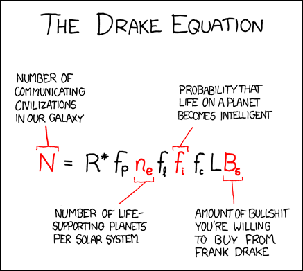
There is a mathematical formula by American Astronomer and Astrophysicist Frank Drake [3]. He is hugely regarded as the father of modern SETI(Search for extraterrestrial intelligence).
The criticism related to Drake’s equation is not about the correctness of the equation itself, but about the highly ambiguous estimations of the various variable used in the equation.
The equation is as follows,
$$N = R^* \times f_p \times n_e \times f_l \times f_i \times f_c \times L$$
Here,
$N$ = the number of civilizations in our galaxy with which communication might be possible (i.e. which are on our current past light cone);
$R*$ = the average rate of star formation in our galaxy
$f_p$ = the fraction of those stars that have planets
$n_e$ = the average number of planets that can potentially support life per star that has planets
$f_l$ = the fraction of planets that could support life that actually develop life at some point
$f_i$ = the fraction of planets with life that actually go on to develop intelligent life (civilizations)
$f_c$ = the fraction of civilizations that develop a technology that releases detectable signs of their existence into space
$L$ = the length of time for which such civilizations release detectable signals into space

For people wondering what is a light cone, here is a picture. This is
a gloried way of looking into the dynamics of time.


In special and general relativity, a light cone is the path that a flash of light, emanating from a single event (localized to a single point in space and a single moment in time) and traveling in all directions, would take through spacetime

---

Criticism:

1. One major setback of this equation is that it takes no account of the cosmological developmental phases and time, the value of $N$ would heavily rely on the speed of cosmological development[1].
2. There is no derivation or methodology of how this equation came into being; which suggests that it is just a stab in the dark.
3. The factor $n_e$ determines habitability; how in the fuck’s world do you find that? Oxygen and Water makes Earth habitable for humans; and probably in some planet $\mathcal{X}$, Nitrogen and Alcohol makes it habitable [2].

---

Here is a beautiful image about Drake’s equation,

---

Conclusion:

1. This is a very badly written equation; not because it is wrong. But, because it has no methodology involved. Looks like couple of fresh college graduates wrote this while having some really potent weed.
   2.Drake’s equation is therefore a Fermi Paradox.

The Fermi paradox or Fermi’s paradox, named after physicist Enrico
Fermi, is the apparent contradiction between the lack of evidence and
high probability estimates, e.g., those given by the Drake equation,
for the existence of extraterrestrial civilizations.

---

An interesting coming from xkcd[3], it added another term $B_6$ which is the amount of bull shit you are gonna buy from the the drake equation.

---

Cheers!

Euler - Riemann Zeta Function.

“Madam, I have just come from a country where people are hanged if
they talk.” ― Leonhard Euler

The Riemann Zeta function, denoted as $\zeta{(s)}$ is a function of a complex variable $s$ that analytically continues the sum of the Dirichlet Series, [1]
$$\LARGE \zeta{(s)}= \sum_{n=1}^{\infty}\frac{1}{n^{s}}$$
The entire blog will be divided into the following parts:

1. What is Analytic Continuation?
2. What is Dirichlet Series?
3. Recurrence relation between Bernoulli Numbers.
4. Relationship between Bernoulli, Riemann and Euler.

---

1.

Before we talk about Analytic continuation, we will have to know what an Analytic function is.

There are multiple ways of defining the Analytic functions[2]. The one that I find most comfortable is given below:
$\underline{\text{Definition 1}}$: A function $f(z)$ is said to be analytic in a region $\mathcal{R}$ of the complex plane if $f(z)$ has a derivative at each point of $\mathcal{R}$ and if $f(z)$ is single valued.

For better understanding, I will extend an example,
$\underline{\text{Example 1}}$: Consider $f(z)$ = $2xy + i(x^{2}-y^{2})$, determine if the given function is analytic or not.
$\underline{\text{Solution}}$: We will use the Cauchy-Riemann equations.

For a given, $f(z) = f(x+iy) = u(x,y) + i v(x,y)$
Now we have the following definitions,
$$u_{x} = \frac{\partial{u}}{\partial{x}}, \\ u_{y} = \frac{\partial{u}}{\partial{y}}, \\ v_{x} = \frac{\partial{v}}{\partial{x}}, \\ v_{y} = \frac{\partial{v}}{\partial{y}}.$$
Now, according to the Cauchy-Riemann Equation, any $f(z)$ is an analytic function, iff,
$$u_{x}=v_{y}, \\ u_{y} = -v_{x}.$$

Now, for the given $f(z)$,
$$u(x,y) = 2xy, \\ v(x,y) = x^{2}-y^{2}.$$
Hence, the relations are,
$$u_{x} = \frac{\partial{(2xy)}}{\partial{x}} = 2y, \\ u_{y} = \frac{\partial{(2xy)}}{\partial{y}}=2x, \\ v_{x} = \frac{\partial{(x^{2}-y^{2})}}{\partial{x}}=2x, \\ v_{y} = \frac{\partial{(x^{2}-y^{2})}}{\partial{y}}=-2y.$$
It is clear that,
$$u_{x} \neq v_{y}, \\ u_{y} \neq -v_{x}.$$
Therefore, the given $f(z)$ is not an analytic function.

Analytic continuation is a pretty simple concept to understand really.
$\underline{\text{Definition 2}}$: Say $f(z)$ is an analytic function defined over a non-empty open subset $W$ of the complex plane $\mathcal{C}$. If $V$ is a larger open subset of $\mathcal{C}$, containing $W$, and $\mathcal{F}$ is an analytic function defined on $V$ such that,
$$\mathcal{F}(z) = f(z), \forall z \in V$$
In other words, Analytic continuation is the method of extending the domain of an analytic function. [3]

For some cool examples on Analytic continuation refer Virginia Tech’s paper here [4].

---

2.

Dirichlet Series[5] is any series of general form,
$$\sum_{n=1}^{\infty}\frac{a_n}{n^{s}}$$
Now, with a slight modification,
$$a_n = 1 , \forall n \in \mathcal{R}$$
We get,
$$\sum_{n=1}^{\infty}\frac{1}{n^{s}}$$
For a function defined as,
$$\zeta{(s)} = \sum_{n=1}^{\infty}\frac{1}{n^{s}}$$
is the Riemann Zeta function.

---

3.

Definitions,[6]
$$s_{0}(n)=n,\\ s_{1}(n) = \frac{n(n-1)}{2},\\ s_{2}(n) = \frac{n(n-1)(2n-1)}{6}...$$
Therefore, $s_{p}(n)$ is given as,
$$s_{p}(n) = \frac{1}{p+1}n^{p+1}-\frac{1}{2}n^{p}+\frac{p}{12}n^{(p-1)}+0 \times n^{(p-2)}+...$$
More generally,
$$s_{p}(n)=\sum_{k=0}^{p} \frac{B_{k}}{k!} \frac{p!}{(p+1-k)!}n^{(p+1-k)}$$
for $n=1$,
$$0=\sum_{k=0}^{p} \frac{B_{k}}{k!} \frac{p!}{(p+1-k)!}$$
or equivalently,
$$B_p=-\frac{1}{p+1}\sum_{k=0}^{p-1} \binom{p+1}{k}$$
The above relation is symbolically written as,
$$(B+1)^{(p+1)}-B^{(p+1)}=0$$
On expansion, all $k$-th powers of $B$, $B^{k}$ must be written as $B_k$ and treated as Bernoulli Numbers.
The expansion is done on the basis of Binomial Theorem, which statest that,
$$\forall a,b \in \mathcal{Z} \ \text{and} \ n \in \mathcal{N}\\ \large (a+b)^{n}= \sum_{k=0}^{n}\binom{n}{k}a^{n-k}b^{k}$$
Therefore, for $n=5$,
$$(a+b)^{5} = \sum_{k=0}^{5}\binom{5}{k}a^{5-k}b^{k}\\ \implies(a+b)^{5} = \binom{5}{0}a^{5-0}b^{0}+\binom{5}{1}a^{5-1}b^{1}+\binom{5}{2}a^{5-2}b^{2}+\\ \binom{5}{3}a^{5-3}b^{3}+\binom{5}{4}a^{5-4}b^{4}++\binom{5}{5}a^{5-5}b^{5}\\ \implies(a+b)^{5} = 1 \times a^{5}b^{0}+5\times a^{5-1}b^{1}+10\times a^{5-2}b^{2}+\\ 10\times a^{5-3}b^{3}+5\times a^{5-4}b^{4}+1\times a^{5-5}b^{5}\\ $$
Therefore, for $(B+1)^{(p+1)}-B^{(p+1)}=0$, after expanding for $p=4$ we have,
$$(B+1)^{(4+1)}-B^{(4+1)}=0 \\ \implies (B+1)^{5}-B^{5}=0 \\ \implies 1\times B_5+5\times B_4+10 \times B_3 + 10 \times B_2 + \\ 5 \times B_1+1\times B_0 =0\\ \implies 1\times 0+5\times B_4+10 \times 0+ 10 \times (\frac{1}{6}) + \\ 5 \times (\frac{-1}{2})+1\times 1 =0\\ \implies 5\times B_4+10 \times (\frac{1}{6}) + 5 \times (\frac{-1}{2})+1 =0\\ \implies B_4=-\frac{1}{30}\\ $$

---

4.

Euler found a formula which easily defined the **even-numbered zeta**functions as follows[7]:
$$\zeta(2n)=(-1)^{(n+1)}\frac{{B_{2n}}{(2\pi)^{2n}}}{2(2n)!}$$
Interestingly, $B_{2n+1}=0 \ \ \forall n \geq 1$, so there is no counter-part for $\zeta(2n+1)$ and yet a value of $\zeta(3)$ exists. Well, that is beyond my scope of this blog.
Cheers!